Finding diurnal cycles in the temperature record at Hargraves Hall - 1
Contents
Read the data and make a simple plot
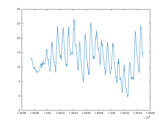
w=webread('http://geoweb.princeton.edu/people/simons/CSV/weather_data.csv');
time=w.x1445486040;
temperature=w.x13_3;
plot(time,temperature)
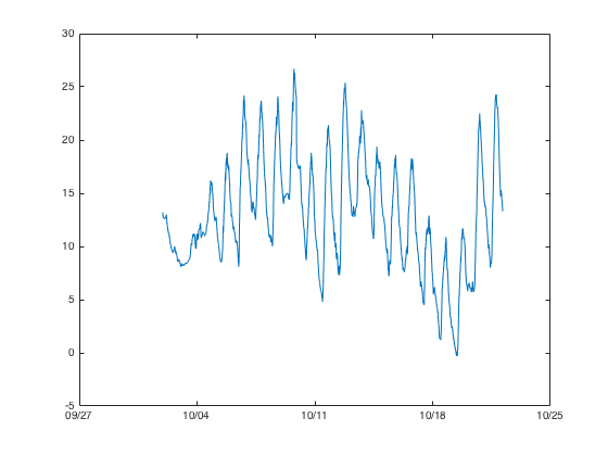
Convert and plot in a human-intelligible format
dates=time/24/60/60+datenum(1970,1,1,0,0,0);
plot(dates,temperature)
datetick('x',6)
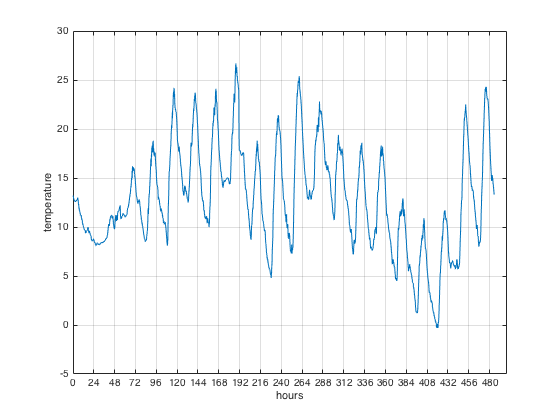
Convert and plot in hours since the first sample which is last
hours=[dates-datenum(dates(end))]*24;
plot(hours,temperature)
set(gca,'xtick',0:24:hours(1))
grid on
xlabel('hours')
ylabel('temperature')
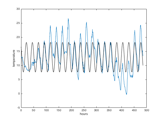
Make a 24-hour sinusoid to overlay on the data
P=24;
A=std(temperature);
m=mean(temperature);
ph=-9.05;
diurnal=m+A*sin(2*pi*[hours-ph]/P);
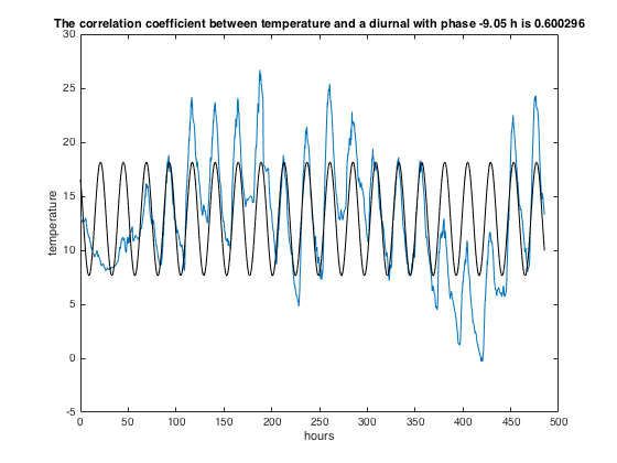
Now make a final-looking plot
clf
plot(hours,temperature)
hold on
p=plot(hours,diurnal,'k');
xlabel('hours')
ylabel('temperature')
Compute the correlation coefficient between the synthetic and the data
[r,pval]=corrcoef(temperature,diurnal);
title(sprintf('The correlation coefficient between temperature and a diurnal with phase %g h is %g',...
		   ph,r(2)))
hold off